Getting started
From a measurement file to your first plot in five minutes. The pictures show a short demo drive: a made-up vehicle with four CAN messages on channel 1.
Prefer to watch?
The same steps, and more, are shown in the tutorial videos on YouTube.
Install
- Download
BusLogAnalyzer_<version>_Windows.zipfrom the latest release. - Extract it to a folder you can write to, such as one in your Documents. The
application keeps its log files and your settings beside itself, so avoid
C:\Program Files. - Run
BusLogAnalyzer.exe.
Windows protected your PC
The application is not signed yet, so Windows SmartScreen may stop it the first time. Click More info, then Run anyway.
The top row
Everything starts from the row at the top of the window, read from left to right in the order of the work.


| Item | What it does | |
|---|---|---|
| 1 | File | Open configuration, Save configuration (Ctrl+S), Export plotted signals (Ctrl+E), Save decoded measurement as MF4, Measurement info (Ctrl+I) |
| 2 | Open Measurement | Opens a BLF, ASC, TRC, MF4, MDF or CSV file (Ctrl+O) |
| 3 | Databases | Assigns DBC, ARXML and LDF databases to the bus channels |
| 4 | Decode | Reads the measurement and decodes it into signals (F9) |
| 5 | Calculated Signal | Creates a signal calculated from others by a formula |
| 6 | Trace | Shows the raw CAN and LIN frames (Ctrl+Shift+R) |
| 7 | Tools | Convert files: join, cut, resample and convert measurements, open or not |
| 8 | Help | This guide (F1), the keyboard shortcuts, where to ask a question or report a problem, the log folder, the user survey and About |
Items you cannot use yet are greyed out. The status bar at the bottom of the window always says what to do next.
1. Open a measurement
Click Open Measurement (Ctrl+O) and choose your file.
For a raw bus log, the application scans the file for its CAN and LIN channels, so that the next step can show them.
Already decoded?
An MF4, MDF or CSV file that holds decoded signals needs no database. Go straight to step 3.
2. Assign the databases
Click Databases. The Database Manager lists the channels it found in the measurement.
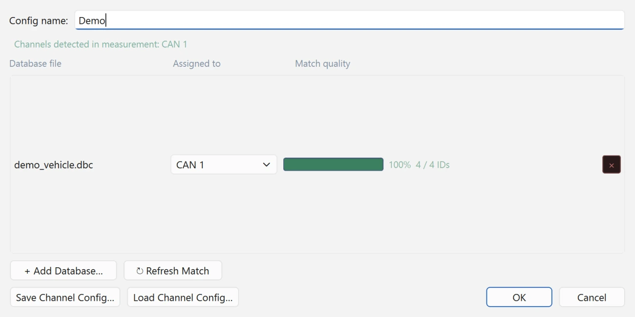
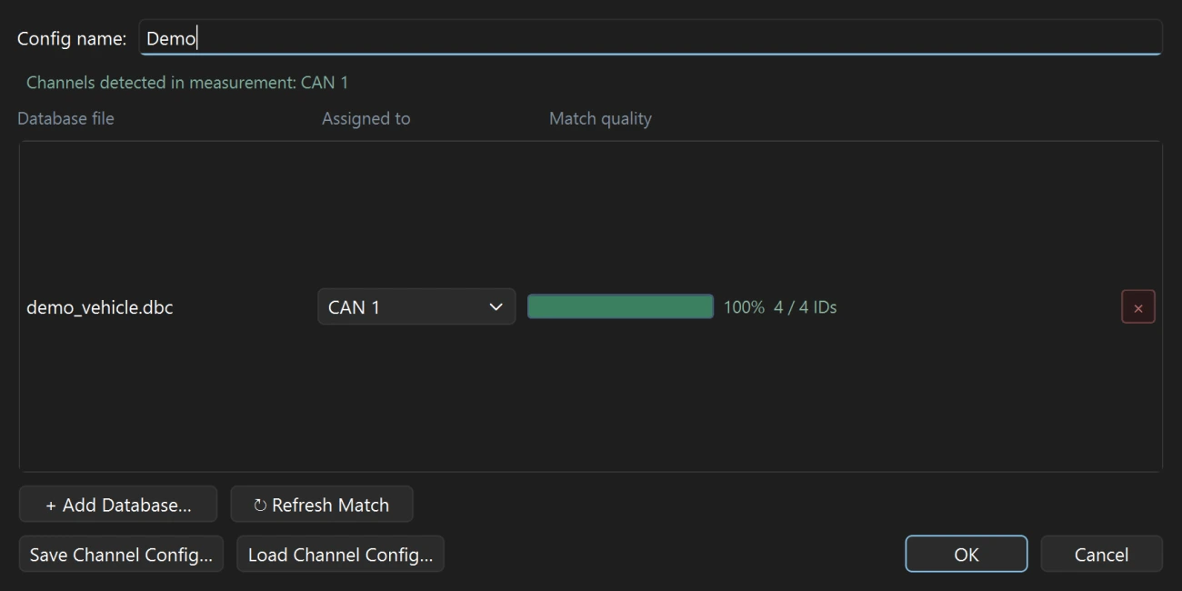
- Click + Add Database… and choose your DBC, ARXML or LDF files.
- Under Assigned to, choose the channel each database belongs to. All CAN (or All LIN) applies a database to every channel of that bus that has no database of its own.
- Check Match quality: it shows how well the database fits the frames on that channel. A low match usually means the wrong channel or the wrong database.
- Click OK.
To use the same assignment again, click Save Channel Config…. Next time, Load Channel Config… restores it in one step.
3. Decode
Click Decode (F9). The status bar shows the progress, and the Log below the plot reports what was read.
When it is done, the signal tree on the left lists every channel, message and signal.
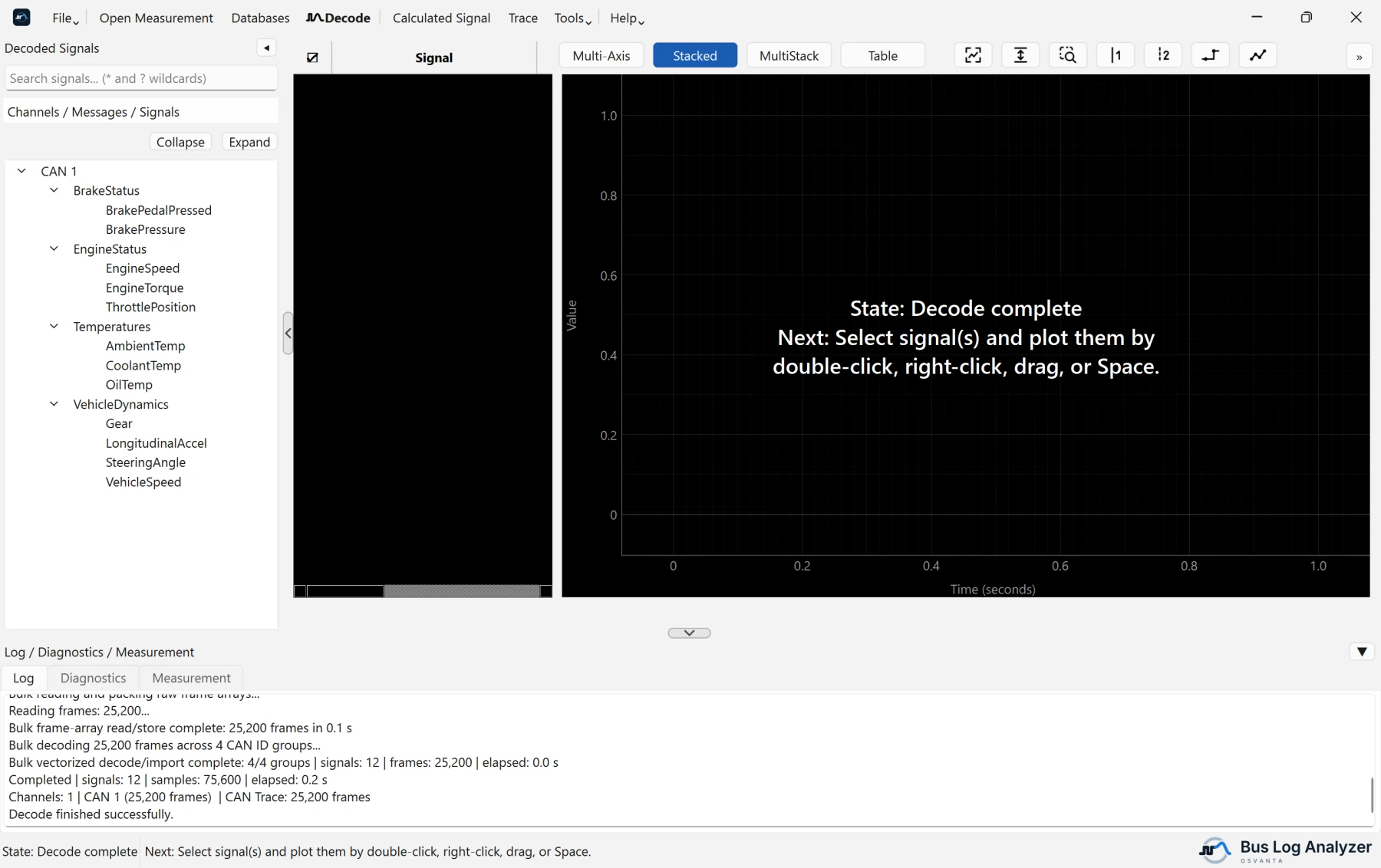
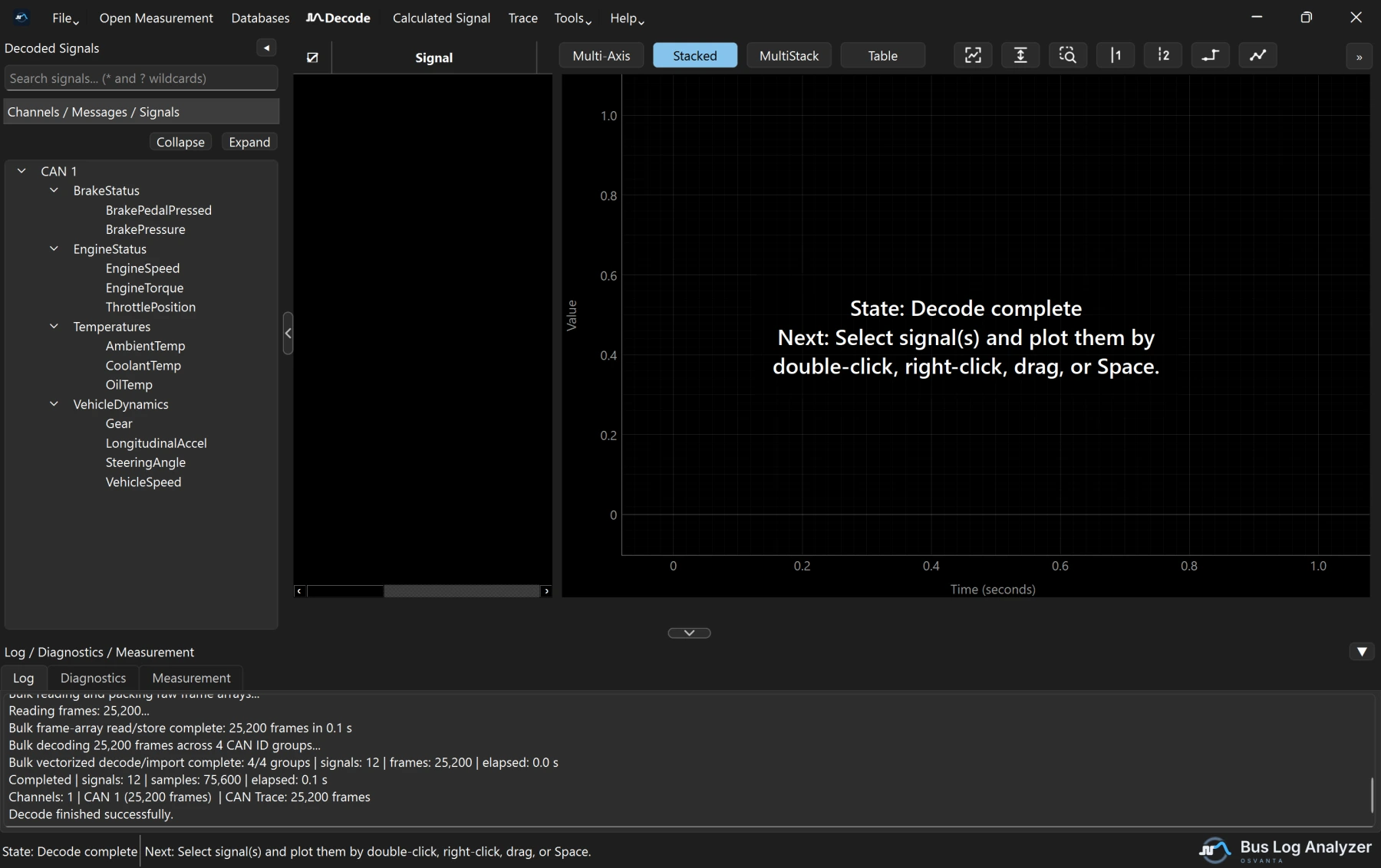
Type in Search signals… to find a signal: the text can be anywhere in its
name, in any case. * stands for any text and ? for one character, so
veh*speed finds VehicleSpeed.
Right-click a signal and choose Properties… to see what the database says about it: its message and ID, start bit, length, byte order, factor, offset, range, unit, value table and comment, and which database file it came from.
File ▸ Measurement info (Ctrl+I) describes the file itself: its format, size, start time and duration, and for an MF4 its header, events and attachments.
4. Plot
Plot a signal from the tree in any of these ways:
- double-click it;
- select one or more and press Space;
- drag them onto the plot;
- right-click them and choose Plot selected signal(s).
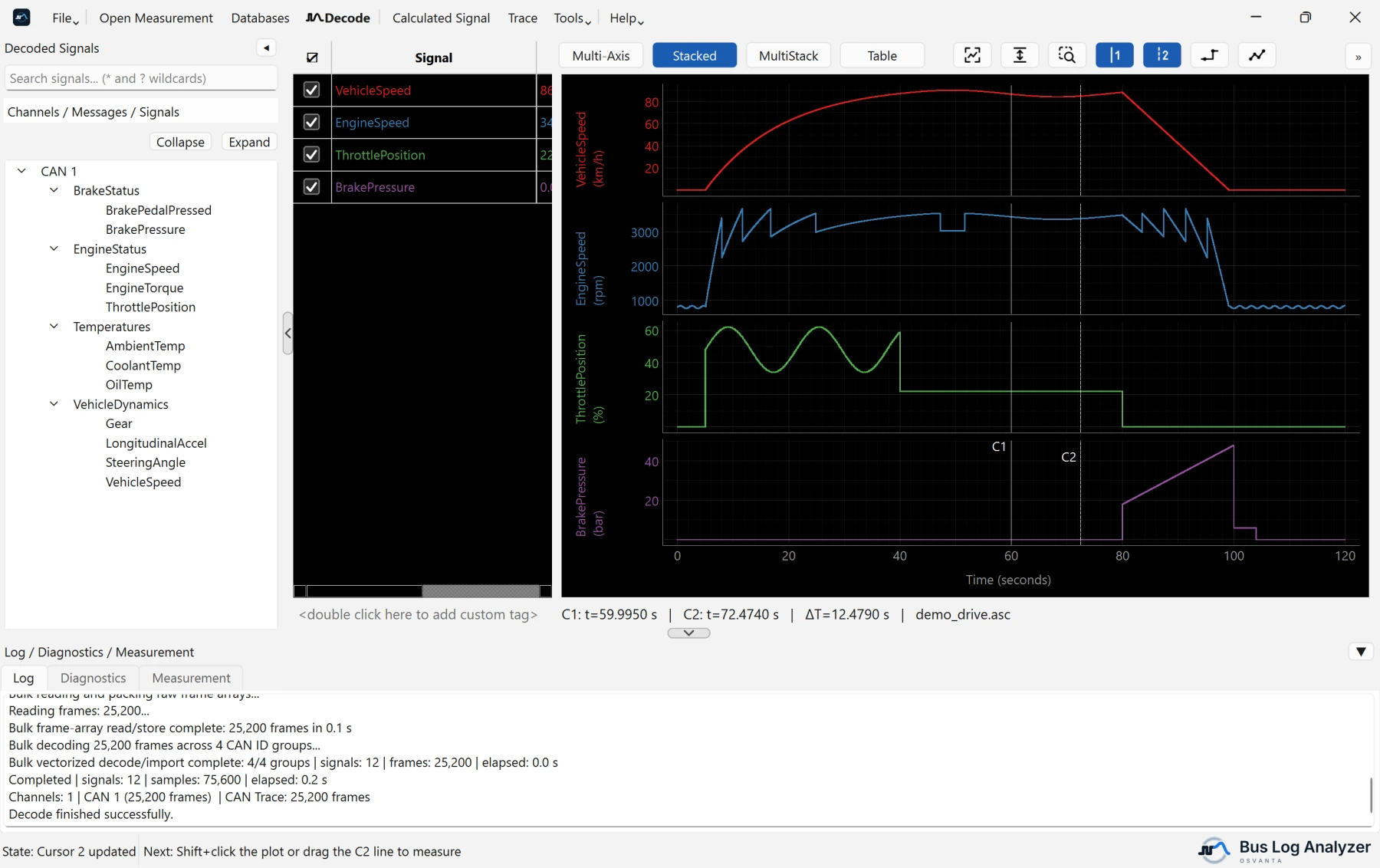
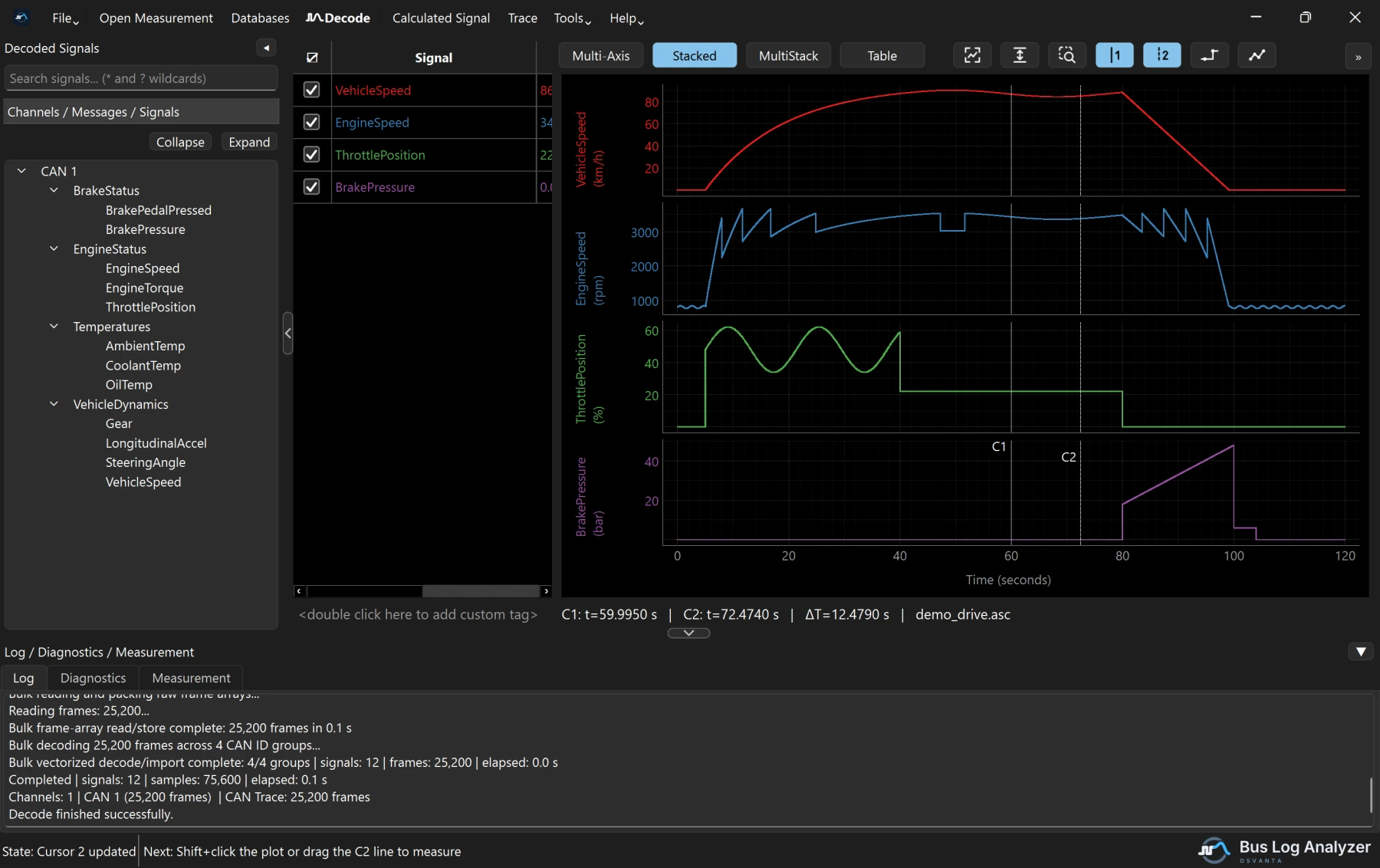
Plot modes, the first three buttons above the plot:
- Stacked, the default, gives each signal its own row and scale.
- Multi-Axis draws the signals over each other, with an axis for each unit.
- MultiStack has rows that hold several signals: drag signals into a row to overlay them. The signal table splits to match: each row gets its own part of the table, level with it and as tall as it, listing only its signals, with a line where one row meets the next. A part with more signals than fit scrolls on its own. Drag a signal from one part to another to move it to that row, or within a part to change its order. Signals of a row whose signals are all unticked are listed under the last row, so they can be ticked back on.
Table, the fourth button, lists the plotted signals as a table beside the plot, a row per sample time.
Tabs. Each tab above the signal table and the plot has its own signals, signal table, plot mode and Table view. + adds a tab, a double-click on a tab renames it, and its small x or its right-click menu closes it; Ctrl+Tab and Ctrl+Shift+Tab move between tabs. Drag signals from the tree onto a tab to plot them there, or onto + to plot them in a new tab. Drag rows from the signal table onto another tab to move them, or right-click them and choose Move to tab. While Synchronize Tabs, the chain-link button, is on, as it is at first, every tab shows the same time range and cursors. Markers, measurement events, the signal table's columns and the line mode are the same in every tab. A configuration keeps every tab, and an older version of the application opens its first tab.
Cursors. A click on the plot places Cursor 1, and Shift+click places Cursor 2. The line under the plot shows both times and the time between them, and the signal table shows each signal's value at each cursor.
Signal table columns. Right-click the table header to show or hide a column: the cursor values, Hex (Cursor 1's value as the raw value on the bus, in hexadecimal), Δ C2−C1 (Cursor 2's value minus Cursor 1's), the unit, and the statistics Min, Max, Mean, Std dev, RMS and Samples. The statistics are between the cursors when both are on, and over the visible range otherwise. A value shown as text, such as a database's "SNA" or a state name, is left out of the statistics and has no Δ; the signal's numbers still count.
Hex turns the value back into what the bus carried: (value − offset) /
factor from the database, padded to the signal's length, so an 11-bit signal
reads 0x7FF and an 8-bit signed −1 reads 0xFF. A float signal shows its
IEEE 754 bits. A signal no database defines (a calculated signal, or an MF4
channel the file decoded itself) shows its value in hex when it is a whole
number, and nothing otherwise.
Signal properties. Right-click a signal in the tree or in the signal table and choose Properties… to see what its database says about it: start bit, length, byte order, factor and offset, range, unit, value table, its message and the database file it came from. Copy puts it all on the clipboard, for a bug report.
Markers. Right-click the plot and choose Add marker here, or press M to add one at Cursor 1. Drag a marker to move it, double-click it to rename it, and right-click it to move Cursor 1 there or delete it. Go to marker in the plot's right-click menu lists them: click a name to bring that marker into view, or the waste bin just after its name to delete it. The list stays open, so several go in a row of clicks, and Del deletes the highlighted one. Delete Markers, the marker and waste bin icon above the plot, offers Delete all markers. Markers are saved in the configuration, and an MF4 export keeps them as events.
Look. Right-click a signal in the table to change its colour (C), give it a line style (solid, dashed, dotted or dash-dot), group it with others, hide it, or remove it. The line-mode button (S) switches between Step Mode, where each value is held until the next sample, and Interpolation Mode, where straight lines join the samples.
Trace. The Δt column is the time since the previous frame with the same ID on the same channel, and the bytes that changed since that frame are bold and coloured; right-click the header to turn either off. While ⇄ Follow Cursor 1 is on, picking a frame moves Cursor 1 to it, and moving Cursor 1 brings its frame into view.
Moving around. F fits the whole recording, and V fits the height only. With Rectangle Zoom (Z), drag a box to zoom into it, Shift+drag to zoom out, and double-click to see everything again. Ctrl+Z undoes the last plot action.
5. Keep your work
- File ▸ Save configuration (Ctrl+S) saves the session to a
.jsonfile: the measurement, the databases, calculated signals, the plotted signals with their colours, groups and order, the axes and the cursors. File ▸ Open configuration brings it all back. - Closing with changes you have not saved asks whether to save them. Whatever you answer, the application keeps the session, and the next start offers to reopen it, even after a crash.
- File ▸ Export plotted signals (Ctrl+E) writes the plotted signals to CSV or Excel, on the time base you choose, or to MF4.
- Tools ▸ Convert files joins, cuts and converts measurements. In
Choose signals, Save as… keeps the ticked signals as a named
selection that works on any file, and Import .txt… and Export .txt…
share a list with others: one signal name a line,
*and?allowed.
Next
- Learn the keyboard shortcuts.
- Something not working? See Help and troubleshooting.